Predicting AirBnB Review Scores: Report

Names:

• Artur Rodrigues, arodrigues (at) ucsd (dot) edu
• Doanh Nguyen, don012 (at) ucsd (dot) edu
• Ryan Batubara, rbatubara (at) ucsd (dot) edu

A website version of this file is available here

Go back to Readme.md as a file

Go back to Readme.md as a website

Table of Contents:

• Predicting AirBnB Review Scores: Report
  • Table of Contents:
  • Introduction
  • Methods
    • Data Exploration:
      • Data Cleaning
      • Whole Dataset Visualizations
      • Numeric Feature Visualizations
      • Non-Numeric Feature Visualizations
    • Preprocessing
      • Missingness and Imputation
    • Model 1
    • Model 2
  • Results
    • Model 1
    • Model 2
  • Discussion
    • Model 1
      • General Metric Discussion
      • Model on Fitting Graph
      • Coefficient Analysis
      • Improvements and Next Steps
    • Model 2
      • Hyperparamter Tuning
      • General Metric Description
      • Model on Fitting Graph
      • Improvements and Next Steps
  • Conclusion
  • Statement of Collaboration

Introduction

Back to table of contents

Since the end of COVID-19, people have been eager to go out of their homes after the long lockdown. Often hesitant to go to more public places like hotels, many may think of AirBnb when seeking more unique, personalized, and private getaway options. As AirBnb users, we wanted to take a deeper look into what makes an AirBnb listing special - in other words, why are some listings rated higher than others? By training a model that can predict a listing’s review scores, we will have a better understanding as customers to what we should look out for in our next booking. For hosts, such a model may help them improve existing listings or predict the popularity of new ones.

Thus, as our model serves a real purpose to both the customer and host, it is important that we make our predictions as accurate as possible while ensuring a large variety of listings and reviews are well-represented. In order to do this, we must first explore the data at hand.

Methods

Back to table of contents

Data Exploration:

Back to table of contents

This project will be based on data gathered by Inside AirBnb May to June 2024. To keep our analysis more focused, we will only be analyzing AirBnB listings from the United States. Since Inside AirBnB only offers datasets per city, we have downloaded all US cities with AirBnB listings and combined them into one csv file.

We now had around 250,000 rows of data and 80 features.

Due to the size of this file, Inside AirBnB reposting policies, and Github Data storage policies, we will not be uploading this combined file to the repository. That said, the combined dataset is available here, but requires a UCSD account.

Data Cleaning

Back to table of contents

After fixing some of the data’s datatypes, we dropped all listing with 0 reviews, since it is not well defined how a NaN reivew score should behave as training data. We then dropped some features that were irrelevant to our project. We show reasons for dropping them below:

• All URL: Unique elements for each listing. Does not contribute anything when predicting the review score.

• All ID: Unique elements for each listing. Does not contribute anything when predicting the review score.

• host_name: Indiviudally unique elements for each listing. Does not contribute anything when predicting the review score.

• license: Unique elements for each listing. Does not contribute anything when predicting the review score.

• source: Holds whether or not the listing was found via searching by city or if the listing was seen in a previous scrape. There is no logical connection between this and the target variable, which is review score.

• host_location: Private information.

• host_total_listings_count: There exists another feature called host_listings_count, this is a duplicate feature.

• calendar_last_scarped: Holds the date of the last time the data was scrapped, no logical connection between this and predicting review_score_rating.

• first & last review: provides temporal data for the first & last review date. Last review date can be misleading as an unpopular listing may have no reviews for an extended amount of time, and suddenly get a review.

• minimum_minimum_nights, maximum_minimum_nights, minimum_maximum_nights, maximum_maximum_nights: The all time minimum and maximum of a listing’s minimum and maximum nights requirement for booking. This has no correlation to review score because you cannot write a review if you have not stayed at the listing.

Further details can be found in this file.

Whole Dataset Visualizations

Back to table of contents

We first show some visuals to demonstrate the sheer size and complexity of our data, starting with our pairplot:

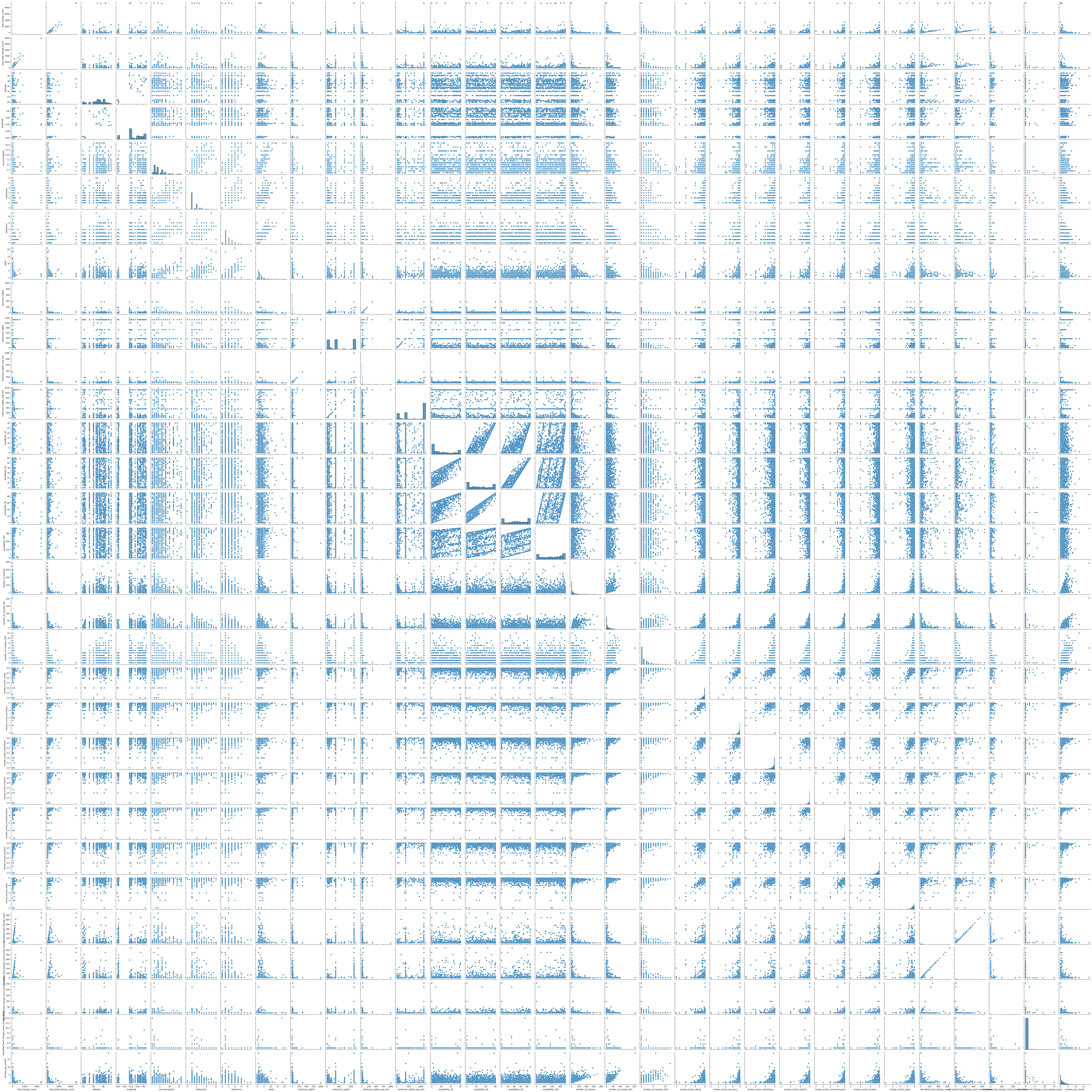
There are many trivial relationships that can be seen in the pairplot, e.g. higher number of listings tends to mean higher number of ratings, or number of beds tends to increase with number of bedrooms, etc.

Also, near the middle of the pairplots we can see a 4x4 square of the availability_365, availability_90, availability_60, and availability_30 features, these plots look very linear which would make sense given that they are all intimately related as subsets and supersets of one another.

We can see this in our correlation heatmap below:

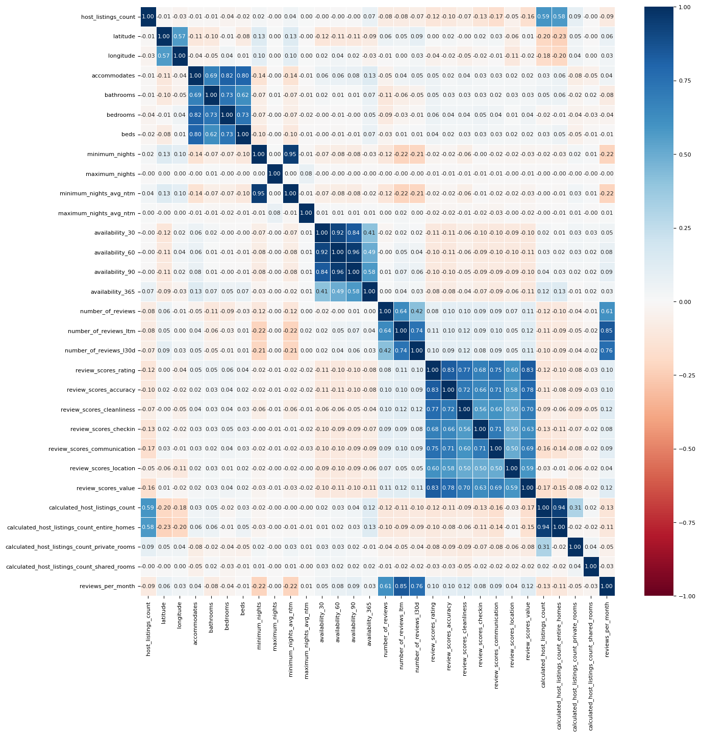
Now, our data appears more tangible, and relationships become more clear. For instance, closer to the middle of the heatmap, we see a 3x3 and a 4x4 square of high correlation features. The 3x3 square shows the correlation between the number_of_reviews, number_of_reviews_ltm (ltm stands for Last Twelve Months), and number_of_reviews_l30d (l30d stands for Last 30 Days) features. It makes sense why these would be highly correlated as number_of_reviews is a super set of number_of_reviews_ltm which is a superset of number_of_reviews_l30d.

Now, in the top left quadrant of the heatmap, we see two 2x2 squares and one 4x4 square of high correlation features. The relatively highly correlated 2x2 square which contains the latitude and longitude features makes sense since we are looking at only listings in the United States and there are areas in the US that are highly population dense relative to the other areas. The other 2x2 square of highly correlated data contains the host_listings_count and host_total_listings_count features which would make sense since in the data dictionary both of these features contain the exact same description.

The high correlation between latitude and longitude is interesting, so we decide to plot the location of all the listings:

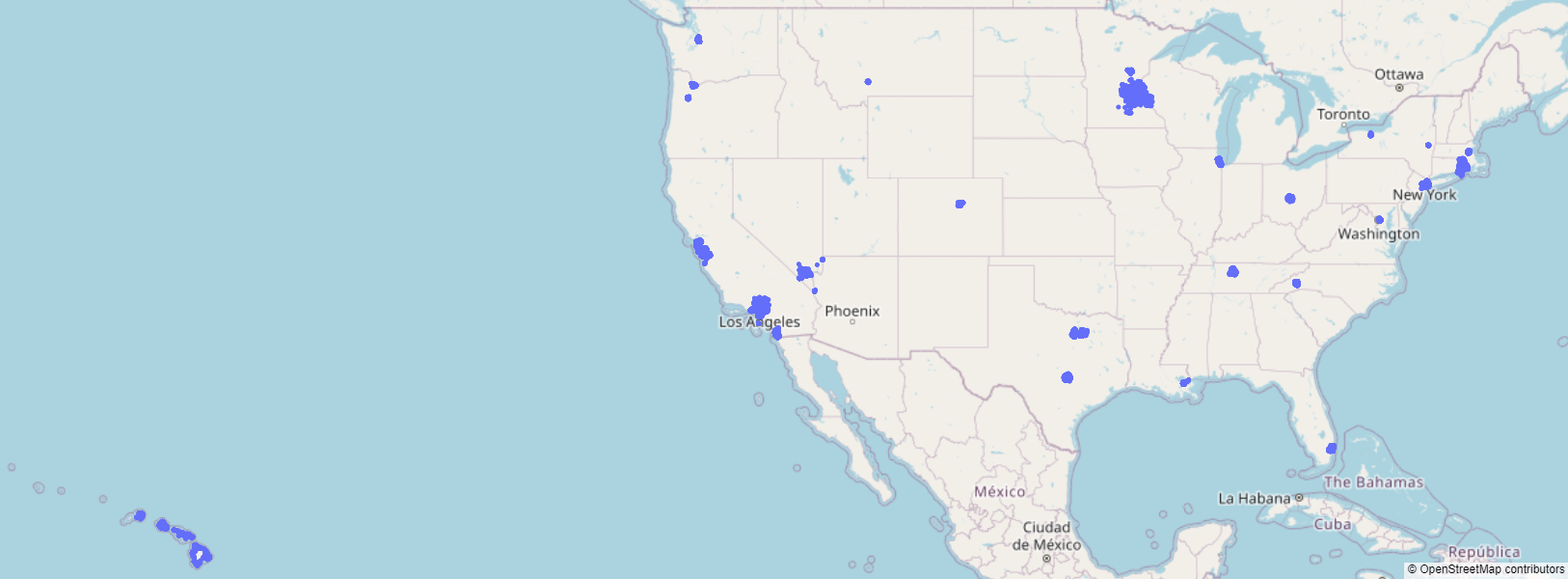
Indeed, listings are prevalent around populous areas - such as New York or Los Angeles - and tourist areas - such as Hawaii.

This high level overview helps us appreciate the scale and complexity of our data, but we need to go deeper to find what features might be useful for the model.

Numeric Feature Visualizations

Back to table of contents

As there are too many features, we only discuss the most interesting ones here. For a more detailed description, see here.

We start by looking at the distribution of all the review scores:

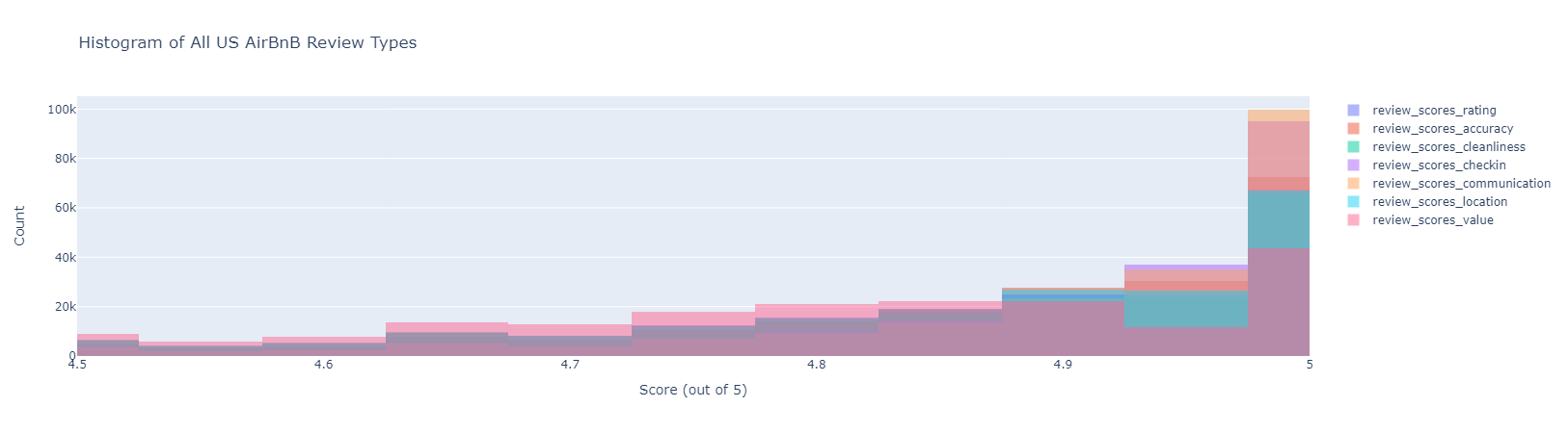
The values actually range from 0 to 5, but we zoom in on this region as >90% of the values are here. Clearly, all of the review scores are very similar. Thus, moving foward, we will use review_scores_rating, the average of all other review features, as our model’s target variable.

One feature we might think is correlated to rating is price:

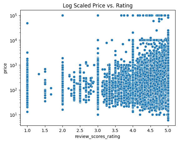
It appears that price increases as the ratings go up, with many exceptions. There does not seem to be any general trend though, except that there are vertical lines where the ratings are integer values - this is probably from all the listings with very small reviews. Even in these lines there is not a general relationship it appears.

In brief, there does not appear to be a single numerical feature with a clear-cut linear or polynomial relationship with review scores. So we turn our EDA to exploring non-numerical columns.

Non-Numeric Feature Visualizations

Back to table of contents

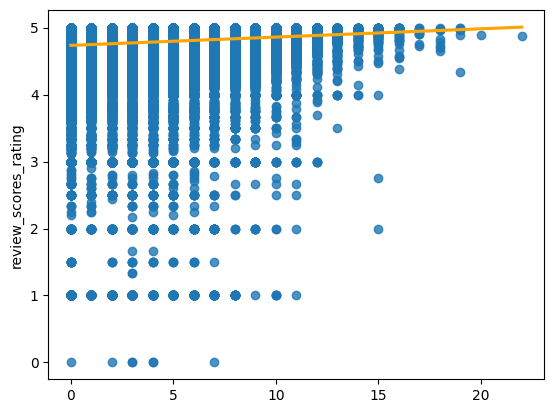
One idea is that a host's age on the platform would overall mean higher ratings (from experience):

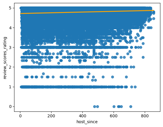
In the above graph, the number of weeks that a host has been on the platform is on the x-axis versus the review_scores_rating feature on the y-axis. We can see a small, but not insignificant, positive correlation between the two, which indicates that the longer a host has been on the platform, the higher their review rating tends to be, but nothing high correlation.

As an aside, it is interesting to see when US hosts signed up for AirBnb:

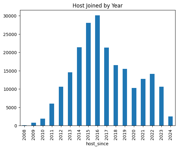
Indeed, our initial guess that AirBnb spiked in popularity due to the pandemic appears to be correct. That is, the platform started to see a surge in the number of hosts signing up at the time, though not as great as the company’s boom in 2015.

Going back to the model, we seek to explore how other non-numerical data relate to review scores. Since many of these features ended up in our final model, we discuss them in the preprocessing section below.

Preprocessing

Back to table of contents

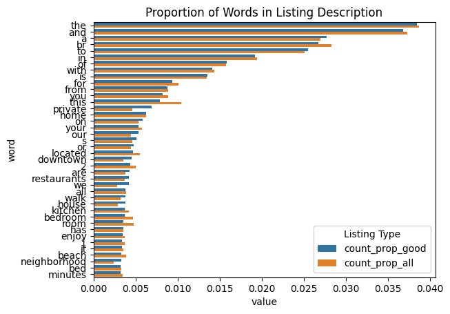
Our dataset contains many text-columns, which we approached by counting the most prevalent words of, and comparing their prevalence amongst all listings versus listings with a 4.9+ rating and at least 100 reviews, which we arbitrarily define as popular listings.

For example, this approach yields us the following visualization for words in the listing description:

We decided to take all the non-filler words, and encode a feature whose value is the number of times these keywords appeared in a listing:

Indeed, this looks like a promising feature, as there is a clear positive slope, and listings with many values are exceedingly rare. Continuing our feature engineering in this direction, we find that this sort of “word counting” trick works for all the text-based features.

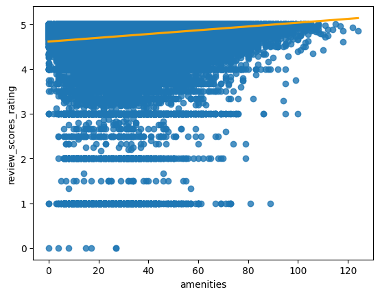
There is one last feature worth mentioning in our feature engineering process: amenities. amenities is a list of host-reported amenities from ‘Jacuzzi’ to ‘Suave Shampoo’. Interestingly, taking the length of this list makes for a pretty good feature:

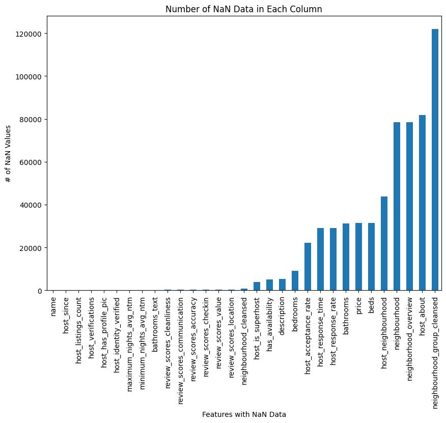
Missingness and Imputation

Back to table of contents

The last step of the preprocessing was to determine what exactly we should do with observations that had missing data. This is actually quite the concern:

For features that were numerical, we decided to take the mean of that feature across all observations and use that to replace the missing data. For categorical, it was a bit trickier. We initially thought that we would take the median observation and replace the missing data with it. But we decided against it since we might be introducing something that a listing did not have originally.

For example, the amenities feature is a list of amenities that consists of all the amenities a listing provides. If we took the most appeared amenity and used it to replace a NaN for a listing, that may or may not even have this amenity, we are essentially adding bias. So we decided to simply ignore this feature if a listing is missing it.

Thus, our preprocessing can be summarized using the following preprocessing sklearn pipeline:

preproc = make_column_transformer(
    (SubstringsTransformer(names_meaningful), 'name'),
    (SubstringsTransformer(desc_meaningful), 'description'),
    (WeekTransformer(), 'host_since'),
    (LengthTransformer(), 'host_verifications'),
    (OneHotEncoder(handle_unknown='ignore'), ['property_type']),
    (OneHotEncoder(handle_unknown='ignore'), ['room_type']),
    (LengthTransformer(), 'amenities'),
    (StandardScaler(), numeric_features)
)

As you can see, amenities is not the only column that gets a special kind of transformer. For more details, see our model.ipynb. We list down some of the more interesting ones not mentioned above:

• Host Verifications: The column host_verifications tells the user which methods of communication the host is verified with. To work with this feature, we decided to encode the length of the list, since it would be difficult to determine whether it is more valuable to have one type of verification than the other, but it is relatively sensible that more verifications imply a more communicative host. We then plotted a regression plot and based on the graph, observed that the relationship between host_vertifications and review_scores_rating is pretty flat, indicating that host_vertification has a weak correlation to review_scores_rating, making it an unreliable feature, hence we are dropping it, i.e. not using it in our model. This makes sense, since someone is unlikely to rate a listing higher just because say the host is accesible through two email adresses instead of one.

• Property Type: When it comes to the property_type feature, we trained a linear regression model using only this feature and when we look at the r^2 score for our model, we get 0.02993098364575919. The r^2 score can be seen as a continuous value in the interval [0, 1] which indicates how good this feature is at helping our model predict the reivew rating for a listing where 0 means bad and 1 means good. The score we got isn’t good but its not like this feature is insignificant either. This is significant, as there are ~125 different property types, so including a OneHotEncoding() of this feature will introduce ~125 new features!

• Host Response Time and Rate: For host_response_time, as we did with room_type and property_type, we used this feature to train a linear regression model and then got an r^2 score, this time of 0.002128186367516438. Similar to room_type this is a very low r^2 score which indicates to us that this feature is not very relevant in our model’s prediction of a listing’s review rating, thus we are not going to be using this feature. This makes sense - there are only four classes of values in this column: within an hour, few hours, a day, and a few days. These tell us almost nothing. For example, a listing that is only popular in the summer may have a host that responds quickly in the summer, but does not even open AirBnb in the winter - such hosts may have a response time of a few days or more despite delivering highly rated listings. Thus, this is an example of a feature that did not make the cut for our model.

• Host Profile Pic: For host_profile_pic, as we did with room_type, property_type, and host_response_time, we used this feature to train our model and then got an r^2 score, this time of 0.0006544772136575228. Similar to room_type this is a very low r^2 score which indicates to us that this feature is not very relevant in our model’s prediction, probably because around 90% of hosts have a profile picture. As a remark, this makes hosts without any profile picture particularly shady!

Hence, with a ludicrous 217,000 rows and 159 features, we are ready to train some models!

Model 1

Back to table of contents

For our first model, we chose Linear Regression for reasons explained in the Discussion section. Linear Regression does not take any hyperparameters besides the features engineered in our preprocessing section above. Thus, the model implementation is very straightforward:

model = make_pipeline(
    preproc, 
    SimpleImputer(strategy='mean'),
    LinearRegression()
)

We then do a 10-fold cross validation using the following code:

X = df.drop(columns=review_cols)
y = df['review_scores_rating']

scores = {}

kf = KFold(n_splits=10, shuffle=True, random_state=42)
for i, (train_index, test_index) in enumerate(kf.split(X)):

    X_train_fold, X_test_fold = X.iloc[train_index], X.iloc[test_index]
    y_train_fold, y_test_fold = y.iloc[train_index], y.iloc[test_index]

    model.fit(X_train_fold, y_train_fold)
    y_train_pred_fold = model.predict(X_train_fold)
    y_test_pred_fold = model.predict(X_test_fold)
    
    scores[i] = {}
    scores[i]['train'] = {
        'mean_squared_error': mean_squared_error(y_train_fold, y_train_pred_fold),
        'mean_absolute_error': mean_absolute_error(y_train_fold, y_train_pred_fold),
        'r2_score': r2_score(y_train_fold, y_train_pred_fold)
    }
    scores[i]['test'] = {
        'mean_squared_error': mean_squared_error(y_test_fold, y_test_pred_fold),
        'mean_absolute_error': mean_absolute_error(y_test_fold, y_test_pred_fold),
        'r2_score': r2_score(y_test_fold, y_test_pred_fold)
    }

Model 2

Back to table of contents

For our second model, we opted for a Sequential Neural Network featuring LeakyRelu activation functions. To choose the hyperparameters, we conducted three grid searches, the first two to reduce the size of the problem space for the third one.

First, we searched through every possible keras optimizer and learning rate order of magnitude:

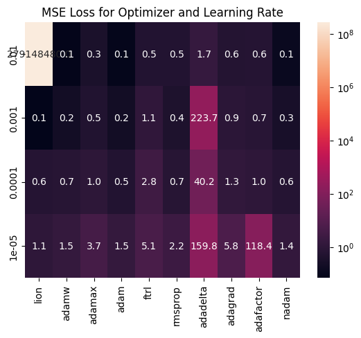
Clearly, Lion, Adam/AdamW, and Nadam have the best, smallest, and most consistent losses, so these are what will move on to our hyperparamter tuning stage. We then see how the number of layers and nodes per layer affect our MSE loss:

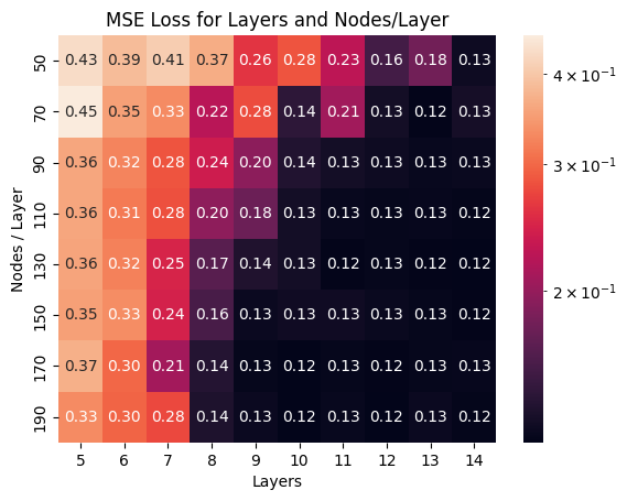
Here, we see how our model’s training loss decreases as we add more layers and more nodes. This is consistent with the fitting graph - as we add more layers or nodes, we increase model complexity, and run the risk of overfitting our training data. This means we need to hyperparameter tune in the region between 8-11 layers and 90-130 nodes, since this is when the loss starts to go down, without it being too high that we run the risk of overfitting.

Thus, we have the following hyperparamters left to tune:

• Optimizer: AdamW, Nadam, or Lion
• Learning Rate: 0.00001 - 0.0001
• Layers: 8-11
• Nodes/layer: 90-130
• Activation Function: relu,sigmoid,tanh (for hidden layers)

Thus, let’s define a Keras Tuner to automatically report the best combination. We remark that code will not take an unfathomable number of resources since we had already dramatically limited the problem scope in the previous two sections.

import keras_tuner as kt
hp = kt.HyperParameters()

def build_hp_NN(hp):
    model = Sequential()
    model.add(Input(shape=(X_features.shape[1],)))

    num_layers = hp.Int('num_layers', min_value=8, max_value=11)
    for _ in range(num_layers):
        model.add(Dense(
            hp.Int('num_nodes', min_value=90, max_value=130, step=10),
            activation=hp.Choice('activation_func', ['relu','sigmoid','tanh'])
        ))
        model.add(LeakyReLU(negative_slope=0.01))

    model.add(Dense(1))

    optimizer_dict = {'lion': Lion, 'adamw': AdamW, 'nadam': Nadam}
    optimizer_class = optimizer_dict[hp.Choice('optimizer_class', ['lion','adamw','nadam'])]
    learning_rate = hp.Float('learning_rate', min_value=1e-5, max_value=1e-3, sampling="log")
    model.compile(
        optimizer=optimizer_class(learning_rate=learning_rate),
        loss='mean_squared_error',
        metrics=['mean_squared_error','val_mean_squared_error']
    )
    return model

The best hyperparameters are as follows:

Hyperparamter	Best Value
num_layers	9
num_nodes	110
activation_func	sigmoid
optimizer_class	lion
learning_rate	5.449514749224714e-05

We thus implement the final tuned NN with the folllowing code:

def make_best_NN():
    """Returns best NN based on hyperparameter tuning."""
    model = Sequential()
    model.add(Input(shape=(X_features.shape[1],)))

    for _ in range(9):
        model.add(Dense(110,activation='sigmoid'))
        model.add(LeakyReLU(negative_slope=0.01))

    model.add(Dense(1))

    model.compile(
        optimizer=Lion(learning_rate=5.449514749224714e-05),
        loss='mean_squared_error'
    )
    return model

We then run 10-fold cross validation to evaluate the model:

scores2 = {}
X_copy = X_features
y_copy = y

kf = KFold(n_splits=10, shuffle=True, random_state=42)
for i, (train_index, test_index) in enumerate(kf.split(X_copy)):

    X_train_fold, X_test_fold = X_copy[train_index], X_copy[test_index]
    y_train_fold, y_test_fold = y_copy.iloc[train_index], y_copy.iloc[test_index]

    model = make_best_NN()

    model.fit(X_train_fold, y_train_fold,epochs=50,verbose=0)
    y_train_pred_fold = model.predict(X_train_fold,verbose=0)
    y_test_pred_fold = model.predict(X_test_fold,verbose=0)
    
    scores2[i] = {}
    scores2[i]['train'] = {
        'mean_squared_error': mean_squared_error(y_train_fold, y_train_pred_fold),
        'mean_absolute_error': mean_absolute_error(y_train_fold, y_train_pred_fold),
        'r2_score': r2_score(y_train_fold, y_train_pred_fold)
    }
    scores2[i]['test'] = {
        'mean_squared_error': mean_squared_error(y_test_fold, y_test_pred_fold),
        'mean_absolute_error': mean_absolute_error(y_test_fold, y_test_pred_fold),
        'r2_score': r2_score(y_test_fold, y_test_pred_fold)
    }

Now that we have implemented our models, we report the results of our 10-fold cross validations.

Results

Back to table of contents

Note: An in-depth discussion of these results and potential improvements can be found in the Discussion Section.

Model 1

Back to table of contents

We do 10-fold cross validation and report the metrics for each fold on our Linear Regression model.

	mean_squared_error	mean_absolute_error	r2_score
(0, ‘train’)	0.12613	0.198191	0.0879473
(0, ‘test’)	0.130564	0.20048	0.08552
(1, ‘train’)	0.127414	0.199016	0.0872061
(1, ‘test’)	0.118979	0.195752	0.0924823
(2, ‘train’)	0.126681	0.198671	0.0875633
(2, ‘test’)	0.125549	0.19663	0.0893076
(3, ‘train’)	0.127029	0.198596	0.0875516
(3, ‘test’)	0.123754	0.197797	0.0795305
(4, ‘train’)	0.126899	0.198766	0.0880649
(4, ‘test’)	0.123835	0.196832	0.0828053
(5, ‘train’)	0.12554	0.197758	0.0881043
(5, ‘test’)	0.135944	0.203179	0.0836539
(6, ‘train’)	0.126947	0.198569	0.0878757
(6, ‘test’)	0.123132	0.198147	0.0866351
(7, ‘train’)	0.126227	0.198311	0.0874304
(7, ‘test’)	0.129676	0.198832	0.0900592
(8, ‘train’)	0.126344	0.198277	0.0879102
(8, ‘test’)	0.128622	0.199914	0.0859053
(9, ‘train’)	0.126359	0.198572	0.0884995
(9, ‘test’)	0.128394	0.198563	0.0812679

We summarize it by taking the averages below:

	mean_squared_error	mean_absolute_error	r2_score
test	0.126845	0.198613	0.0857167
train	0.126557	0.198473	0.0878153

We also attach the average differences between each metric’s train and test:

	mean_squared_error	mean_absolute_error	r2_score
difference	-0.000288	-0.000140	0.002099

Model 2

Back to table of contents

We do 10-fold cross validation and report the metrics for each fold on our Sequential Neural Network model.

	mean_squared_error	mean_absolute_error	r2_score
(0, ‘train’)	0.100324	0.166675	0.187977
(0, ‘test’)	0.130965	0.177124	0.0920074
(1, ‘train’)	0.101551	0.179577	0.196185
(1, ‘test’)	0.101345	0.179156	0.149704
(2, ‘train’)	0.100578	0.175928	0.200441
(2, ‘test’)	0.107871	0.177049	0.130703
(3, ‘train’)	0.102913	0.18821	0.192934
(3, ‘test’)	0.100765	0.191031	0.0704145
(4, ‘train’)	0.103356	0.182372	0.185835
(4, ‘test’)	0.103187	0.184251	0.092417
(5, ‘train’)	0.102092	0.182962	0.207228
(5, ‘test’)	0.0919273	0.18137	0.0514895
(6, ‘train’)	0.0991111	0.170512	0.187944
(6, ‘test’)	0.138846	0.182306	0.119488
(7, ‘train’)	0.100006	0.174586	0.187665
(7, ‘test’)	0.121794	0.185548	0.177905
(8, ‘train’)	0.103255	0.172554	0.187263
(8, ‘test’)	0.0966669	0.172099	0.143063
(9, ‘train’)	0.0995553	0.173294	0.204133
(9, ‘test’)	0.122812	0.188462	0.057875

We summarize it by taking the averages below:

	mean_squared_error	mean_absolute_error	r2_score
test	0.111618	0.18184	0.108507
train	0.101274	0.176667	0.19376

We also attach the average differences between each metric’s train and test:

	mean_squared_error	mean_absolute_error	r2_score
difference	-0.010344	-0.005172	0.085254

This concludes our results.

Discussion

Back to table of contents

We split the discussion into three subsections for each model:

1. General Metric Discussion
2. Model on Fitting Graph
3. Improvements and Next Steps

Model 1

Back to table of contents

We start by motivating why we start with linear regression. Linear regression is a hyperparameterless model - besides feature engineering. This means the model has 3 main benefits:

1. It is relatively simple, and features almost entirely dictate how well the model performs. This allows us to focus on enginnering good, relevant features for our second, more complicated model.
2. Linear Regression allows us to check the coefficient of every variable, and when standardized or normalized, a sense of which features play the largest role in determining the review score.
3. It is extremely fast and easy to implement LinearRegression, allowing us to test many different features and encodings quickly.

General Metric Discussion

Back to table of contents

Our mean absolute error for our linear regression was 0.19 for both the train and test prediction. The similarity between these values tell us that our model has not overfitted, but the large values (considering review ratings go from 0 to 5 only) show us that the model is not very good. Same can be said for mean squared error which was 0.12.

The r2_score however tells a very interesting story. The r2_score is a correlation metric that goes from 0 to 1, where 0 implies no correlation and 1 is identical correlation. Our low value of 0.08 tells us that despite the large number of features, we still have not effectively represented the data.

In conclusion, our first model did not perform very well. Our data is too sporadic and that attempting to fit a simple line on data that is complex is fruitless no matter how often we optimize our coefficients (which is the only way we can optimize in linear regression), scaling a line would only result in a line.

Model on Fitting Graph

Back to table of contents

Since our MSE is high, and since the complexity of linear regression is very low, we are simply underfitting our data. Again, we are attempting to fit a line on data that is sparse and not very linear. Based on our relatively high MSE, and generally almost identical test and train MSE, MAE, and r2, it is safe to say that our model is not that far along the fitting graph. In other words, our model has not overfitted the data since we see very similar values between the test and train metrics. This is very good for us, as there is much room to add more model complexity - such as by adding more features, or changing to a more complex model - and improve the metrics in our second, better model.

Coefficient Analysis

Back to table of contents

Recall that one of the main reasons we chose Linear Regression for our first model is the ability to compare the significance of various features to the regression. We summarize the values of the absolute values of our coefficients:

Description of Coefficients	Value
count	159.000000
mean	0.021966
std	0.028256
min	0.000027
25%	0.004170
50%	0.009904
75%	0.030899
max	0.153812

We notice the average value is 0.021, meaning our columns do have an impact on the review score to the 0.01 order of magnitude. Then, to identify the features that contributed most to our regression, we can sort the features from largest to smallest absolute value coefficient. Here are the top 10 features (as indexes) and their coefficients:

154 0.153812 63 0.130499 86 0.126531 155 0.116383 90 0.112651 93 0.103163 88 0.096587 130 0.076349 87 0.075408 101 0.067546

In order to do more in-depth coefficient analysis, we need to look at what each column actually represents (not just their indexes). Using our pipeline, we list down the columns:

• 1 substring feature (from name)
• 1 substing feature (from description)
• 1 week feature (from host_since)
• 1 length feature (from host_verifications)
• 125 one-hot encoded features (from property_type)
• 4 one-hot encoded features (from room_type)
• 1 length feature (from amenities)
• 25 numeric features (as listed in numeric_features)

We discuss the top ten features below (citing their index as well):

• Feature 154 (calculated_host_listings_count): It makes quite a lot of intuitive sense why this feature would be the most impactful, the more reviews a host has, the more likely it is that one of their listings is going to be a high rating listing. The longer a host is on the platform, the more time they have to accumulate reviews. This is definitely a feature that we could try to feature engineer further to give our model more to work with.

• Feature 155 (number_of_reviews_l30d): The number of reviews a listing has in the last 30 days seems to have played quite a significant role in the model’s predictions. This makes sense as, similar to calculated_host_listings_count, the more reviews a listing has in the last 30 days, the more likely that listing is to have a good rating since people wouldn’t want to keep booking and reviewing a place that is poorly rated.

• Feature 130 (some room_type): We see that there is a room type that reigns supreme over all of the other room types. This would make sense as AirBnB is a service that offers practical temporary housing, so people who just need a quick place to recharge and rest are in need of a specific kind of room rather than the other possible room types.

• Feature 63, 86, 90, 93, 88, 87, 101 (some property_types): These features are part of our one hot encoded feature property_type, so we know that there are specific property types that are weighted very heavily. This, once again, makes a lot of sense since most users are only going ot be in search of a handful of different property types, rather than there being a uniform distribution over the 125 property types.

Improvements and Next Steps

Back to table of contents

Here are some ways in which we may be able to improve our model:

• Increasing the number of features
• Better feature engineering
• Trying different complexity models such as polynomial regression or neural networks
• We could try using coalesced features.

Since our mean squared error of our first model being linear regression is not exactly ideal, we decided that the next potential model we can train and test would be a neural network. Since the fit of the linear regression line is producing an unoptimal mean squared error, we believe that a simple linear best fitting line is simply not good enough to fit our relatively complex data. By using a neural network and messing around with the amount of neurons per hidden layer, the amount of hidden layers, and the many activation functions, we add more depth and complexity in hopes of finding the best fit that captures the relationship between our features while in turn producing a fairly accurate prediction.

Model 2

Back to table of contents

Our first model has taught us a few things:

• We need to dramatically increase model complexity.
• There is no “magic feature” that is extremely correlated with review scores.
• Many of our features have only a small number of possible numerical values.

As such, a neural network comes to mind for our second model. Here are three reasons why a neural network appears to be the next best step:

1. The data and features are extremely complicated, so simple kernels like linear or polynomial transformations is insufficeint to describe a feature’s relationship with the review scores. By using a neural network, we gain access to the use of activation functions, allowing us to add non-linearity and complexity to our model to better fit our data.
2. We have an incredible number of features (159), and NNs excel at finding general patterns from a large number of features and combining them together (this means we will need a lot of layers with a lot of nodes each).
3. The data is extremely large, meaning that there is much room for our model to explore the data before it overfits. This reduces the high complexity downside of NNs.

Hyperparamter Tuning

Before discussing the results, we remark that through 100 trials of hyperparameter tuning, which took hours, it concluded that the most optimal neurons per layer is 110, optimal hidden layer is 9, optimal activation function is sigmoid, and optimal learning rate is 5.449514749224714e-05. We ended up with a mean squared error of 0.09 - an improvement over our linear regression model. More details can be found in our Methods section.

General Metric Description

Back to table of contents

We start with the mean_absolute_error, which tells us that on average our predicted rating is about 0.17 off for both the test and train cases. The similarity between these values tell us that our model has not overfitted, and though the values are a noticeable improvement compared to our first model, it is not ideal either. This shows how complex predicting review scores is.

Same can be said for our mean_squared_error. We note that its value is smaller than the mean_absolute_error, being on average 0.10, which makes sense as it is roughly the square of the mean_absolute_error.

The r2_score however tells a very interesting story. The r2_score is a correlation metric that goes from 0 to 1, where 0 implies no correlation and 1 is identical correlation. Our value of 0.19 for train and 0.10 for test shows that our data is right on the edge of the fitting graph, meaning it is on the verge of overfitting. This is a marked improvement to our linear regression r^2 of about 0.8, meaning our second model is a definite improvement.

Model on Fitting Graph

Back to table of contents

Based on the similarity of our MSE and MAE, we know that our model has not overfitted the training data. However, the large difference between r2_scores tells us that our model is much futher along - or more complex - than our linear regression model on the fitting graph. In other words, adding more layer or complexity may run the risk of overfitting, though we are clearly not there yet. This is very good for us, since it means that our model is quite generalizable (as the 10 folds contain similar values), but also quite difficult as adding large amounts of complexity is likely going to cause us to overfit our data.

Improvements and Next Steps

Back to table of contents

Compared to our first model, the second model has much higher model complexity, and there is evidence (as discussed in the r2_scores above) that we are approaching the overfitting mark, though we are not there yet. This leaves us at a rather difficult stalemate: We have engineered a lot of features, have a large amount of data, and high model complexity, with optimized hyperparameters and a very small learning rate. This means that any potential model improvements probably needs to involve a major change in how we do our model.

Here are some ways in which we may be able to improve our model:

• Changing the type of NN or NN layers. Right now, we have a “default” NN with backpropagation and only Dense layers with LeakyRelu in between. Perhaps trying different and more complicated layers such as convolution or pooling layers may better bring out the correlations in the data.
• Changing the type of activation function. Mathematically, each activation function is ideal for a very specific type of identification. Perhaps changing activation functions between layers may help bring out the patterns in the data.
• Doing more feature engineering. Some features, such as amenities, are only explored by length. Though it can be argued that there isn’t much for us to do here, (since how much does amenities, for example, really impact the reviews of a listing?), it also means we have not tapped into this data’s full potential. However, a full NLP stack will be necessary for this, which comes with concerns of overfitting and bias.

Conclusion

Back to table of contents

In this project, we trained two models: First a linear regression model, which prompted us to engineer features for categorical columns, and second a neural network, which gave us the model complexity and the ability to hyperparameter tune, allowing us to improve our metrics. Though our best model (the tuned NN) has an MSE of 0.1, MAE of 0.1, and r2 of 0.2, which is not ideal roughly speaking, this is already quite good in the grand scheme of things.

In other words, our purpose of providing more information to AirBnB customers for what things to look out for a highly rated (i.e. enjoyable) stay, and AirBnb hosts by what things to work on to deliver better rated experiences (i.e. more profitable listings) has largely been achieved by this model. For the customer, one can take a listing they really like, but say with 0 or very few reviews, and use the model to heuristically predict whether this listing has the characteristics and potential to be a good stay. For the host, one can take a couple new listings and predict roughly whether one will do better than the other in terms of review scores. This may also allow hosts to tune their descriptions, pricing, etc and predict how these things will impact the review rating of their listing.

Thus, we conclude that given our metrics, being able to predict a given listing’s review score plus minus 0.1 stars is more than enough precision to provide meaningful insights to both parties, and thus the project is largely a success. We note, however, that based on personal experiences, that a 0.1 rating difference can be quite substantial, especially when so many choices are presented to the customer by AirBnb.

We had extensively described potential next steps in the previous section, but the general gist is to try a new type Neural Network with more in-depth engineered features, as predicting AirBnb review scores is more complicated than it seems!

Statement of Collaboration

Back to table of contents

Our group participated in a lot of collaboration. Rather than having clear cut roles, we divvied up the work and did what was expected of us while getting constant feedback from the other group members. This means that while the general descriptions of what we did can be seen below (note: this is not an exhaustive list), we were all very involved with the other group member’s work as well, which means each one of us got a holistic hands-on experience with the entire project and had even participation throughout the whole project. Overall, we were all very involved in the project, and constantly communicated with each other.

• Ryan Batubara: Feature Engineering, Plotting and Graphing, Report Writing, Model tuning, README, Model Design, Exploratory Data Analysis (Plotting), etc.

• Artur Rodrigues: Feature Engineering, Explanations for Plots and Graphs, Report Writing, Banners, Exploratory Data Analysis (Descriptions), etc.

• Doanh Nguyen: Feature Engineering, Explanations for Plots and Graphs, Report Writing (Major Role), Exploratory Data Analysis (Descriptions), etc.

Thank you for reading our project report. Back to table of contents